A PivotTable in Two Minutes

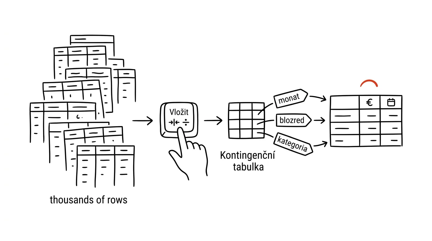
A PivotTable sounds like an advanced feature for analysts, but it's actually one of the fastest ways to turn thousands of rows of raw data into a clear summary. You don't need formulas or macros — just tell Excel what you want to total and how you want it broken down, and the table builds itself. PivotTables aren't for experts — they're for anyone with more than a hundred rows of data.

A typical scenario

David gets a sales export for the whole year — over ten thousand rows with date, product, amount, and region. He needs to know how much was sold each month and in which region. By hand, he'd have to filter the data by month, add up the selected rows, and copy the result into another table — starting over from scratch every time the filter changes.

With a PivotTable, he inserts the data in one step and drags three fields into place: Month into Rows, Region into Columns, Amount into Values. A revenue breakdown by month and region is done in under two minutes, and if new data comes in, the table refreshes with a single click.

How to do it

1. Click anywhere in the source data (Excel figures out the table's boundaries on its own) and go to Insert → PivotTable.
2. Confirm the proposed data range and where to place the new PivotTable (a new sheet is usually the clearest choice) → Enter.
3. In the field list on the right, drag whatever you want to total (say, Amount) into the Values area, and whatever you want to break the data down by (Month, Region, Product) into the Rows and Columns areas.
4. The PivotTable builds instantly and recalculates every time you change the fields you've dragged in — trying out different breakdowns of the data takes seconds.
5. Double-clicking any number in a finished PivotTable opens a new sheet with all the source rows that went into that total — useful for verifying where a number came from.
6. When the source data changes or new rows are added, right-click inside the PivotTable and choose Refresh — the summary recalculates without you having to rebuild it.

The best tools

• Excel's built-in PivotTable — covers the vast majority of summary and reporting needs, with no extra data prep.
• Power Pivot — an add-on for when you need to connect several tables at once or work with millions of rows that would make a regular PivotTable slow.
• Google Sheets — also offers pivot tables, via Insert → Pivot table; the idea of dragging fields into rows, columns, and values is the same.

What you get out of it

• Time: roughly 30 minutes a week compared with manually filtering and summing data every time you need a different view of the same numbers.
• Fast answers to new questions: rearranging fields takes seconds, so when someone asks “what does this look like by product instead of region,” you can answer right away, not tomorrow.
• Lower risk of error: Excel computes the totals from the actual data, not a manual filter and calculator, where rows easily slip through.

Pro tip

A PivotTable linked to a formatted table (Ctrl+T) expands automatically on the next refresh whenever new rows are added to the source — you don't have to adjust the source range by hand every time.